Tutorial#
The purpose of this tutorial is to show new users how to get started with x_epi. In the first part of the tutorial, we will show how you can use x_epi to create the sequence used in Figure 2 of our paper. Then in the second part of the tutorial we will show how you can use x_epi to reconstruct the data acquired using the sequence created in part one.
Sequence Creation#
For this tutorial, we will use the GUI to create the sequence. To launch the GUI, type x_epi_gui in a command prompt and click ‘Use Default’ in the prompt that comes up. This will load the default sequence, which is a multi-echo 3D symmetric EPI sequence with three different metabolites.
General Settings#
As the sequence used in the paper is a single-echo 3D symmetric EPI sequence with only two metabolites, a few changes will have to be made to the default sequence. In the ‘General’ tab, make the following changes:
Change the metabolite field from 3 to 2
Reduce the number of repetitions from 2 to 1
Uncheck the Alternate Polarity: Slice button
Under timing change Exc. Time to 1500 and Set Time to 0
Change the Orientation to Coronal
Reduce the number of echoes form 5 to 1
Under options, switch Ramp Samp. from On to Off.

Changes in the General settings#
Metabolite Settings#
You will need to make specific changes for each of the two metabolites that will be acquired. To do this, first click on the ‘Metabolite’ tab. This will show the current settings for the first metabolite. To match the paper sequence, you will need to make the these changes:
Increase the flip angle to 90 degrees.
Change the metabolite name from ‘pyr’ to ‘eg’ for ethylene glycol
Reduce the partial Fourier fraction in the ‘slice’ direction to 0.66
To change the settings for the second metabolite, you will need to select ‘Met 2’ in the Metabolite dropdown at the bottom of the screen. Then you can make the following changes:
Add a frequency offset of -365 Hz
Increase the flip angle to 90 degrees
Change the metabolite name from ‘lac’ to ‘me’ for methanol
Decrease the acquisition grid from 20x20x20 to 16x16x16
Turn off Partial Fourier in the second phase encoding direction by changing the ‘slice’ partial Fourier fraction to 1
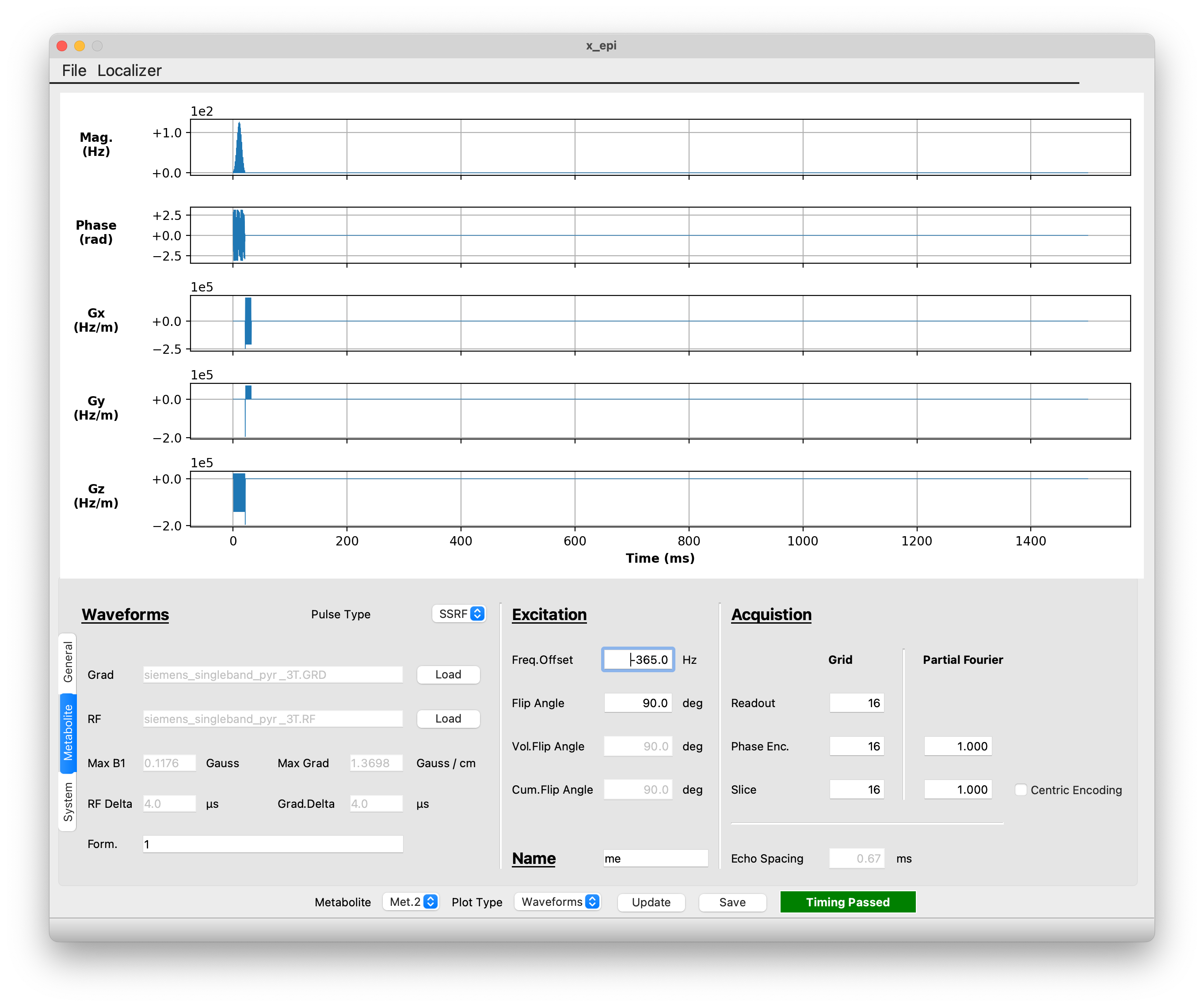
Changes for the second metabolite#
Output#
Once all the necessary changes have been made, you can save the sequence by clicking the ‘Save’ button. For the purposes of this tutorial, we will save the sequence as ‘x_epi_tutorial’. As discussed in the GUI documentation this will produce three difference files. The ‘x_epi_tutorial.seq’ file is the file that will be taken to the scanner and run. If you do plan to test the sequence on your scanner, make sure to switch the image orientation to ‘Coronal’ in the interpreter sequence. If you don’t do this, the reconstructed image will not have the correct orientation. The sequence parameters are listed in ‘x_epi_tutorial.json’. This file can be loaded into the GUI for future editing, and is needed to reconstruct the data.
Reference Scan#
Because symmetric EPI sequences are sensitive to gradient delays between odd and even k-space lines, it is often useful to acquire a reference scan with no phase encoding gradients. You can create a sequence for collecting a reference scan by changing the ‘Phase Enc’ in the General tab to ‘Off’. For the paper, we also changed the flip angle to 45 degrees and frequency offset to 0 Hz for each metabolite. This was done because we acquired the reference scan on the 1H channel.
Once you have made the necessary changes, save the sequence as ‘x_epi_tutorial_ref’
Image Reconstruction#
Once you have acquired data using the a x_epi sequence, you can reconstruct it using the x_epi_recon command line program. You can find an example 13C MRI dataset acquired using the sequence above at our Github. This dataset was acquired using a 3D printed Shepp Logan metabolite phantom containing ethylene glycol (left chamber) and methanol (right chamber). Once you have downloaded the datafile ‘raw.dat’ you can reconstruct it with the following command:
x_epi_recon raw.dat tutorial.json recon -n_avg 32
The second argument is the JSON file describing the sequence used to acquired the data, and the third is the root for each output file. The command will produce a NIfTI image for each metabolite. In this case the output name for each image will be recon_<met_name> where <met_name> is the name given to the metabolite when the sequence was created. The -n_avg 32 flag is added because 32 averages were acquired at the scanner.
If you have a higher resolution structural image, you can pass it with the -anat argument:
x_epi_recon raw.dat tutorial.json recon -n_avg 32 -anat anat.nii.gz
This will create FSL style transformation matrices between each metabolite and the anatomical image using the NIfTI headers.
Finally, you can add in the reference scan data, raw_ref.dat, to account for odd/even timing differences:
x_epi_recon raw.dat tutorial.json recon -n_avg 32 -anat anat.nii.gz -ref raw_ref.dat tutorial_ref.json
The image below shows the output from the recon using a reference scan. The ethylene glycol metabolite image is shown in purple/green/yellow and the methanol image is in purple/orange/yellow. Under both images is a T1-weighted structural image. As expected, the 13C metabolite signal from each metabolite is confined to a single chamber. For more advanced reconstruction options, including POCS and field-map based distortion correction, see the paper and the Github.
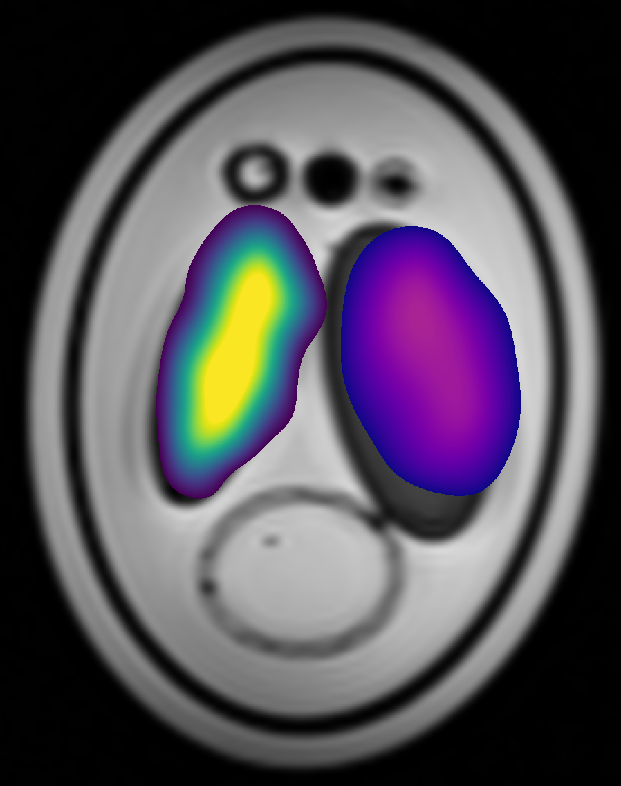
Reconstructed 13C metabolite images#